A Short Cut Method for Evaluating Molecular Sieve Performance

This Tip of the Month shows how a Short Cut Method (SCM), after one Performance Test Run (PTR), may be used to estimate the life of a Type 4A molecular sieve dehydrating a water-saturated feed of natural gas.

The May 2015 Tip of the Month [1] discussed the benefits of standby time.  In that Tip (which the reader is urged to revisit), a case study was presented for a 3-tower dehydration system. The system was designed to meet a three-year life; however, a PTR after one year of service predicted the total life of the molecular sieve would only be about two years. Using the available stand-by time, the molecular sieve life was extended to about 3.7 years.

The above results were calculated used the concepts outlined in Chapter 18 of Gas Conditioning and Processing, Volume 2: The Equipment Modules (9^th Edition) [2]. Due to the non-linearity of the modeling techniques, the manual calculations are tedious. The June 2016 Tip of the Month [3] showed how a computer module developed for the PetroSkills-John M. Campbell GCAP (Gas Conditioning and Processing Software) [4] could be used to perform the same calculations. Among other things, the GCAP module directly calculates the life factor, F_L, which generates more consistent results compared to visually reading the Generic Molecular Sieve Decline Curves (Figure 1).

 

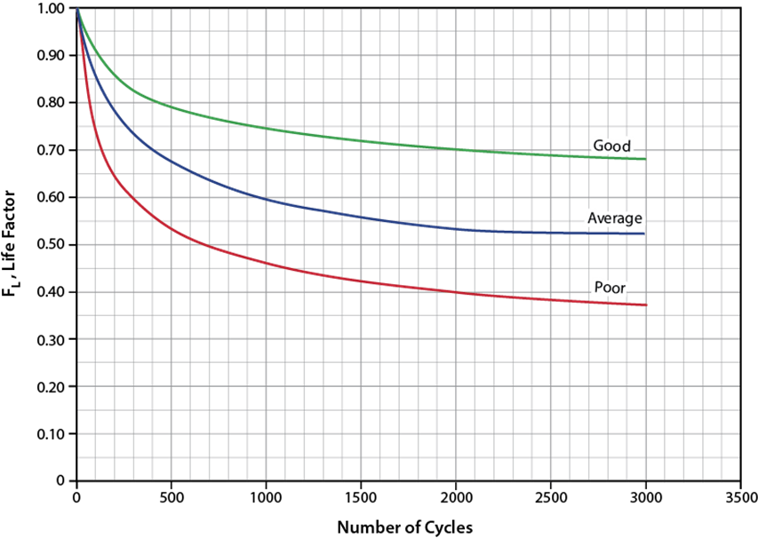
Figure 1. A generica molecular sieve decline curves [1]

 

SHORT CUT METHOD (SCM):

By making a few simplifying assumptions, manual calculations can be performed on the back of an envelope. This SCM permits an operator or a facility engineer to quickly determine the life expectancy of the molecular sieves. The assumptions, which cover the majority of natural gas dehydration units in the field, include:

1. Water-saturated natural gas is the feed

2. The feed conditions remain relatively constant throughout the life of the molecular sieve system

3. Type 4A-1/8 inch (3 mm) pellets or 4×8 beads are used

4. The fresh equilibrium loading is 23 weight percent water

5. The residual loading is 4 weight percent water

6. 5 % of the bed weight is devoted to the Mass Transfer Zone (MTZ)

7. Normal life degradation following the curve shapes in Figure 1. If upsets such as liquid carryover, bed lifting, bed support failure, valve hang-ups, contaminants in the regeneration gas, flow channeling or other adverse conditions occur, the shape of the curves in Figure 1 will be quite different.

Chapter 18 of Gas Conditioning and Processing, Volume 2: The Equipment Modules (9^th Edition) [2] contains equations that permit us to calculate the total mass of the molecular sieve, the Break Through Loading (BTL, or Useful Loading), and the aged net equilibrium loading. Using the assumptions listed above together with the equations in Chapter 18 it can be shown that:

F_L = BTL/18                                                                                                    (1)

where:

F_L        = Life factor

BTL      = (100)(mass of water removed/mass of molecular sieve)                 (2)

The remainder of this Tip of the Month will compare the results of the SCM to those obtained from the rigorous manual method and the computer-generated method.

 

SCM vs RIGOROUS METHOD:

Figure 2 shows the Process Flow Diagram used for the Case Study [2]. Tables 1 gives the Design Basis.  Table 2 presents the Design Summary. Table 3 shows the Results of the PTR after one year of operation (note the feed flow rate and the temperature during the PTR are slightly different than the design basis).

 

Figure 2. Typical process flow diagram for a 3-tower adsorption dehydration system [2]

 

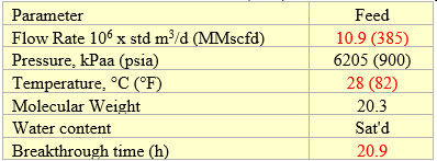
Table 1. Design basis for the case study

 

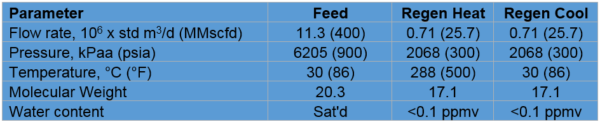
Table 2. Design Summary for the case study

 

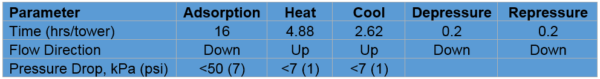
Table 3. Results of Performance Test Run (PTR) after 12 months of operation

 

Additional information used in the Case Study:

• 3 tower system (2 towers on adsorption, 1 on regeneration)
• External Insulation
• Tower ID = 2.9 m (9.5 ft)
• Each tower contains 24630 kg [54300 lb_m] of Type 4A 4×8 mesh beads and is designed to last three years.
• Regeneration circuit capable of handling an extra 15% of flow
• Unit is operated on fixed time cycles
• No step-change events such as liquid carryover, poor flow distribution, etc.

 

Following is a recipe for using the SCM:

1. Use Equation 2 to calculate the design BTL = 10.6 wt %

• • BTL =100 (16 h)(163 kg water removed/h)/(24630 kg mol sieve) =10.6%
  • BTL =100 (16 hr)(360 lb_m water removed/hr)/(54300 lb_m mol sieve) =10.6%

2. Use Equation 1 to calculate the design F_L = 10.6/18 = 0.59

3. Locate the design F_L at 1095 cycles on Figure 3, Calculated Life Factors (F_L=0.59 & 3 years of 24-hour cycles per tower is equivalent to 1095 cycles).  This is the Design F_L Point.

4. Use Equation 2 to calculate the PTR BTL = 12.0 wt %

• • BTL =100 (20.9 h)(141 kg water removed/h)/(24630 kg mol sieve) =12%
  • BTL =100 (20.9 hr)(312 lb_m water removed/hr)/(54300 lb_m mol sieve) =12%

5. Use Equation 1 to calculate the PTR F_L = 12/18 = 0.67

6. Locate the PTR F_L at 365 cycles on Figure3, Calculated Life Factors (F_L=0.67 & one year of 24-hour cycles per tower is equivalent to 365 cycles).  This is the PTR F_L Point.

7. Because the PTR F_L Point falls on a curve lower than the Design F_L Point, we need to be concerned.  Interpolating and extrapolating the capacity decline curve from the PTR F_L Point_, we see an F_L of 0.67 (the Design F_L) will occur after a total of about 750 cycles. This is approximately one year shorter than the expected life.

 

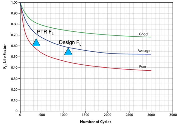
Figure 3. Calculated Life Factors

 

Because the unit has a regeneration circuit that can handle an additional 15% of flow, the complete regeneration cycle (heating, cooling, de- and re- pressurization) can be reduced to 7.0 hours.  This allows the beds to turn around faster. Using the reduced cycle time (the complete cycle time is now 21 hours vs the original 24 hours) and the original design basis conditions with the SCM recipe:

1. Calculate End of Life BTL = 9.3 wt % (from Equation 2).

• • BTL =100 (14 h)(163 kg water removed/h)/(24630 kg mol sieve) =9.3%
  • BTL =100 (14 hr)(360 lb_m water removed/hr)/(54300 lb_m mol sieve) =9.3%

2. Calculate End of Life F_L = 9.3/18 = 0.52 (from Equation 1). This is because less water is being adsorbed per cycle.

3. Interpolating and extrapolating from the PTR F_L Point, we find the End of Life F_L of 0.52 occurs around 1400 cycles (see Figure 4).  Since 365 cycles have already occurred and going forward a reduced cycle time will be used, the molecular sieves are forecast to last a total of 3.5 years.

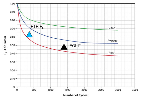
Figure 4. Calculated Life Factors Using Standby Time

 

Table 4 compares the results of the SCM to the rigorous manual calculations (May 2015 Tip of the Month) and the computer-generated calculations (June 2016 Tip of the Month).

 

Table 4. Comparison of Three Methods

 

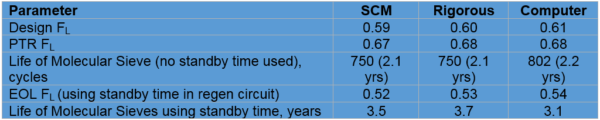
The difference between the predicted life using standby time shown by the Computer Model and the two manual methods is primarily due to the inherent inaccuracy of trying to interpolate and extrapolate data plotted on Figures 3 and 4.  The computer model will produce the same result every time.  This cannot be said when visually reading Figures 3 and 4.   Figure 5 shows the output from the GCAP Computer Model [3]. Note that when working on one curve, the higher the calculated EOL F_L, the fewer the Number of Cycles (NOC) remaining until the beds need to be replaced.

The PTR in the above Case Study was run after 365 cycles.  The slope of the curve is fairly steep in this region and small changes in data can have a significant impact on the life predictions.  While the user can get a good indication of the state of decline of their molecular sieve unit, scheduling additional PTR’s is highly recommended. Finally, generic curves are used in these Figures. The shape of your specific molecular sieve capacity decline curve may differ from these generic curves.  Despite these caveats, the SCM offers the user a quick and easy way to assess the capacity decline of their molecular sieve unit.

 

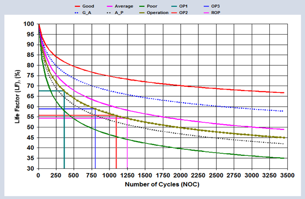
Figure 5. Projected life factor (L_F = 54.3% and NOC = 1251.4) if standby time is used

 

SUMMARY:

We can draw the following conclusions from this case study:

• The short-cut method presented allows the user to quickly estimate the decline of their adsorbent based on only one performance test run for molecular sieve dehydrators using low-pressure regeneration. This permits the early formulation of a credible action plan. The short-cut method compares reasonably well to the rigorous manual approach and the computer-generated model which also require only one performance test run.
• Both manual methods rely on a visual interpolation and extrapolation of the generic molecular sieve decline curves. The computer-generated approach provides much more consistent results.
• All the methods presented in these Tips of the Month rely on open-art technology. The molecular sieve vendors use proprietary methods specific to their manufacturing techniques. Consequently, the results of the approaches presented in these Tips of the Month should be used to generate trends as opposed to absolute values.
• Site-specific factors will determine your unit’s decline curve.  Conducting more than one performance test is highly recommended.
• Standby time offers a large degree of operating flexibility because the decline curves tend to level off; always try to build in standby time in any new molecular sieve design.
• Adsorption capacity is a function of the number of cycles, not calendar time.
• Install a good filter coalescer or filter separator upstream of your adsorption unit to keep the contaminants out of the system.

To learn more about similar cases and how to minimize operational problems, we suggest attending ourG4 (Gas Conditioning and Processing) and PF-4 (Oil Production and Processing Facilities) courses.

 

Written by: Harvey H. Malino, P.E.

---

References

1. Malino, H.M., http://www.jmcampbell.com/tip-of-the-month/2015/05/benefits-of-standby-time-in-adsorption-dehydration-process/, PetroSkills – John M. Campbell, 2015

2. Campbell, J.M., “Gas Conditioning and Processing, Volume 2: The Equipment Modules,” 9^th Edition, 3^nd Printing, Editors Hubbard, R. and Snow–McGregor, K., Campbell Petroleum Series, Norman, Oklahoma, 2018.

3. Moshfeghian, M.  http://www.jmcampbell.com/tip-of-the-month/2016/06/projecting-the-performance-of-adsorption-dehydration-process/, PetroSkills – John M. Campbell, 2016

4. GCAP 9.2.1 Software, PetroSkills – John M Campbell “Gas Conditioning and Processing Computer Program,” Editor Moshfeghian, M., PetroSkills, Katy, Texas, 2016.