

Onshore Gas Gathering Systems – Concept Selection, Basic Design & Operation (Part 3)
Onshore Gas Gathering Systems – Concept Selection, Basic Design & Operation
By: Mark Bothamley
Part 3
Non-metallic flowlines
There are several “non-metallic” options for gas gathering system applications. To a large degree, non-metallics eliminate the corrosion concerns – both internal and external – associated with metallic – typically carbon steel – pipelines.
The non-metallic flowline options that are typically used in gas gathering systems include:
1. High density polyethylene (HDPE), often referred to as “plastic” pipe. Normally used for low pressure gas gathering systems only. Quite commonly used in coalbed methane applications. HDPE will not be discussed further in this article.
2. Spoolable Composite Pipe (SCP).
SCP typically consists of:
1. An inner thermoplastic liner (usually HDPE).
2. One or more reinforcing layers – glass/aramid fibers, or steel.
3. An outer “protection” layer (usually HDPE).
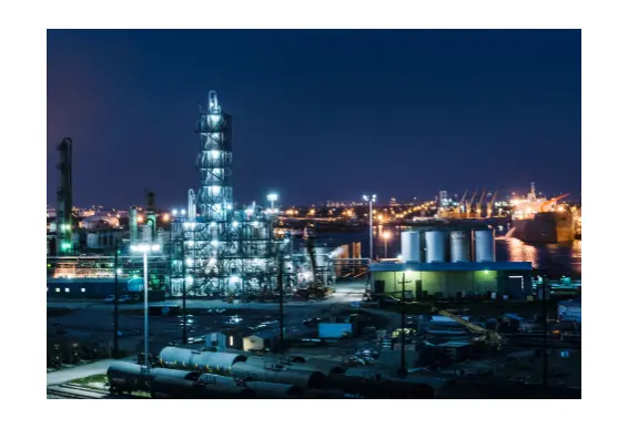
See Figure 12.
Figure 12 Spoolable composite pipe being installed

Some of the main manufacturers/products include:
1. Fiberspar.
2. Flexpipe.
3. FlexSteel.
4. Soluforce.
Available sizes typically range from 2 – 8”, with design pressures as high as 1,500-3,000 psig, depending on the product and diameter. Design temperature limits of 140 F are typical, though some manufacturers offer products with higher temperature ratings. Depending on pipe diameter, 1,500 – 5,000 feet of pipe can typically be accommodated on a single spool.
The primary advantage of SCP – compared to steel – is the potential for significantly reduced life cycle cost. Savings are achieved through lower installation costs, mainly related to the faster laying of the spoolable material, and reduced operating costs associated with the material’s corrosion resistance – internal and external. The smoothness and corrosion resistance of the internal liner typically also leads to lower friction factors and thus reduced pressure drop compared to equivalent steel pipelines, though this is mainly a secondary benefit.
Due to the size limitation of SCP – less than or equal to 8” depending on the product – utilization of this material may sometimes be limited to lower flowrates, eg. individual well flowlines and/or lower capacity trunklines. For high capacity systems, the smaller diameter SCP lines can be connected to larger diameter steel pipelines, or much more rarely to “stick” pipe composite pipelines. Stick pipe composite – generally fiberglass reinforced plastic (FRP) pipe – is available in large diameters, but would not typically be used in moderate to high gas gathering or transmission service.
There are also some downsides to the use of composites in general:
1. Pressure rating dependency on time and temperature is less well defined than steel.
2. Typically more fragile and subject to damage during installation.
3. There can be issues associated with gas permeation through the inner liner, especially at high pressure.
While the advantages of SCP outweigh the disadvantages in most applications, the utilization of SCP for gas gathering in the upstream oil and gas industry is still fairly limited. Its use has been increasing in recent years but there remains some hesitancy to move away from steel, which has provided mostly good experience for a long time.
Line Sizing
This is another large subject area.
The sizing of gas gathering system lines is usually a compromise. For a given flowrate and composition, bigger pipe costs more, but it will generally have a lower frictional pressure drop. For GGS applications this often means less backpressure on the wells and therefore higher well flowrates. However, larger pipe diameters – and the associated lower velocities – also typically have more problems related to liquid holdup/unsteady multiphase flow, eg. slugging, and potentially, solids deposition.
Most conventional/shale/tight gas wells produce gas with liquid contents (at typical in-situ pipeline flowing conditions) in the range of 5 – 50 BBL/MMSCF. A small percentage of gas fields fall outside of this range. Some very high H2S fields produce quite low amounts of hydrocarbon liquids, but at high pressure and low temperature also result in significant volumes of liquid-phase H2S.
Given the number of variables involved – including changing conditions over time – the typical uncertainties associated with many of these variables, and the fact that pipe is available in discrete sizes (and large differences in cross-sectional flow area) it is probably not worthwhile to attempt to size lines to three-decimal place accuracy or allocate much time to selection of the latest multiphase flow code and/or simulator. Figure 13 is an example of a line sizing chart that the author uses for conceptual design work. The chart is based on the modified-Flanigan method which basically provides an adjustment factor to a dry gas flow equation based on the amount of liquid in the line, and also includes a simple liquid holdup calculation to account for terrain effects. For each pipe diameter covered – 2, 3, 4 and 6” – two lines are shown: a “dry gas” line and a line that represents 50 BBL/MMSCF of hydrocarbon liquid at flowing conditions. An “eyeball” interpolation can be performed for liquid contents between 0 and 50 BBL/MMSCF. This particular chart is for a nominal operating pressure of 500 psig. Other assumptions are shown in the Figure. Of course, more rigorous sizing methods should be used when warranted.
Figure 13 Example GGS line sizing chart
|
|

Line Sizing Criteria
Various line sizing criteria have been proposed and used over the years, mainly based on allowable velocity and/or allowable pressure drop guidelines. Often these guidelines are simple rules-of-thumb and may be fine for a given application, if their basis is understood.
While the information presented in Figure 13 is only approximate, some interesting observations can be derived from it. For example,
1. The dry gas lines show only frictional losses. The 50 BBL/MMSCF lines show combined frictional (including liquid effects) and hydrostatic liquid accumulation affects (where the pressure drop lines begin to flatten out and eventually curve upwards with decreasing rate, assuming somewhat hilly terrain.
2. The dashed red ellipse indicates suggested preferred operating conditions which avoid the liquid loading regions and yet also minimize pressure drop due to excessive friction. Operating pressure drops of 15-25 psi/mile are indicated. This is a reasonable value and agrees with other published guidelines in the literature. Lower pressure operation, eg. 100-300 psig would likely warrant a design pressure drop in the 10-15 psi/mile range. Larger diameter, longer, higher capacity trunk lines would also typically be designed for somewhat lower pressure drops.
3. Each line size has fairly narrow capacity ranges between the liquid loading and high friction loss regions, especially the smaller diameters, ie. 2” – 4”.
4. There are some significant gaps in flowrate coverage evident. For example the 10-15 MMSCFD flowrate range is too high (frictional losses) for a 4” line, but too low (liquid accumulation effects) for a 6” line. As 5” pipe is not really an option, other factors would have to be taken into account to allow a selection between 4” and 6” to be made, eg. near future changes in flow and/or pressure. Generally speaking, for multiphase applications higher velocity is better.
Provisions for Future Drawdown/Reduced Pressure Operation to Maximize Deliverability and Reserves Recovery
Deliverability
Figure 14 shows conceptual deliverability curves for a conventional gas well and a shale/tight gas well, with flowing tubing pressure (Ptbg) on the vertical axis rather than the more traditional bottomhole flowing pressure (Pwf). These curves combine the reservoir flow characteristics with a tubing pressure drop calculation for the given operating conditions. This “surface IPR” is more useful when discussing the effects of surface facilities/gathering system options. 29 www.markbothamleyconsulting.com
Figure 14 Typical well “surface” IPR (excluding liquid loading effects at low rates)
|
|

|
Bothamley |
For relatively high permeability conventional reservoirs, gas wells reach a “pseudo-steady state” producing condition where the well drainage region is effectively bounded – usually by adjacent well drainage areas – and average reservoir pressure declines with depletion. The surface IPR curve represents a point-in-time relationship between flowrate and flowing pressure, described by the reservoir parameters used in the radial flow equation and the parameters used to describe the tubing string, eg. inside diameter, measured/true vertical depth, etc. As reservoir pressure (PR) declines with time, the IPR curve drops as well – Figures 16 and 17. Notice the time parameter for the various curves in the two charts. The well deliverability curve “decreases” much quicker for the shale gas well even for minimal change in the static reservoir pressure. This behavior is mainly a reflection of the “flush” high production from the well’s stimulation treatment fractures and the very near rock surface adjacent to the fractures. The native permeability of the shale, which is very low, becomes limiting in a relatively short period of time. Early life prediction of flowrate vs tubing (and gas gathering system) pressure for shale gas wells can be difficult.
The IPR relationship and prediction of reservoir pressure decline can be combined with assumptions re: well/pad site facilities, gathering system configurations and compression timing/location to estimate well and field production rates and pressures vs time. As mentioned previously, an Integrated Asset Model can be very useful for performing the network-wide nodal analysis modeling and time-stepping (to capture reservoir depletion) calculations typically required.
Figure 16 Change in IPR vs time (conventional well example)
|
|

|
Bothamley |
Figure 17 Change in IPR vs time (shale gas well example)
|
|

|
Bothamley |
The shale/tight gas well IPR presented in Figure 14 would seem to indicate that the well’s flowrate is relatively insensitive to back-pressure. This behavior is typical of tight (low permeability) reservoir wells. However, experience gained from existing shale gas developments has indicated that these wells are in fact quite sensitive to surface facilities back-pressure, at least after the initial rapid decline period (Figure 17). This sensitivity is probably more related to liquid loading effects combined with the effect of pressure on gas density and velocity in the well tubing string, as opposed to the effect of flowing bottomhole pressure on reservoir deliverability (see Figure 18). In many shale gas plays, flowrates have declined to < 1 MMSCFD within 2-3 years. Flowing tubing pressure ranges of 100 – 300 psig are typical for most shale gas field developments. These pressures can be achieved via pad-located compression or gathering system compression, depending on the system configuration.
Both conventional and unconventional gas wells can experience reduced - or complete loss – of deliverability due to liquid loading at low flowrates. This is typically a late-in-life effect for conventional wells but may occur fairly early in the life of unconventional wells due to their rapid decline rate. While there are various artificial lift options available to deal with liquid loading, the impact of surface facilities on flowing tubing pressure is an important consideration. Lower backpressure on the wells helps inflow performance and also increases gas velocity in the tubing for a given mass or standard volumetric flowrate of gas.
Figure 18 Typical minimum stable gas flowrates for liquid unloading
|
Bothamley |

Reserves Recovery
The effect of GGS pressure on flowing well tubing pressure – and ultimately reservoir pressure – on recovery is fairly straightforward, at least for conventional “volumetric” reservoirs, with minimal aquifer pressure support. For these reservoirs, ultimate reserves recovery is directly related to reservoir abandonment pressure, as shown in Figure 19 for a hypothetical reservoir. The actual abandonment pressure will be dictated by minimum economic production rates for individual wells and the development as a whole.
Simplistically, recovery for a volumetric gas reservoir can be described as follows:

Figure 19 Effect of pressure on reserves recovery (volumetric reservoir)
|
|

Well flowing tubing pressure and gas gathering system pressure are not the same thing, with the key factors being the location of compression – if utilized – and well flowline/gathering line pressure drop. Tight gas reservoirs have pressure-reserves relationships similar to conventional reservoirs with the gas volumes lower due to generally lower porosity. Shale gas reservoirs behave somewhat differently. They contain both “free” gas and adsorbed gas. The free gas volume is similar to the gas volumes in conventional and tight sand reservoirs but the adsorbed gas volume behaves differently. Similar to coalbed methane reservoirs, quite low reservoir pressures are required to recover the adsorbed gas fraction from shale reservoirs.
System Architecture
For the purposes of this article “system architecture” will be taken to mean the arrangement of gathering lines, compressor stations, etc., connecting the wells/well pads to the receiving gas plant. There are a wide variety of architectures possible due to the number of variables involved, including:
i) Geographical dimensions of the gathering area/reservoir.
ii) Acreage dedicated to the GGS.
iii) Individual vs pad drilled wells and locations of well/pad sites, ie. well/pad spacing.
iv) Well deliverability and pressure vs time.
v) Wellstream composition.
vi) Hydrate prevention strategy.
vii) Liquids handling strategy.
viii) Topography.
ix) Ambient temperature.
x) Provisions for compression.
xi) Facilities ownership.
xii) Etc.
Iqbal outlines some potential gas gathering system layout options (Figure 20), including high-level pro’s and con’s.
Figure 20 Potential gas gathering system layout options.
|
|

Iqbal, Worley Parsons
While there are a fairly large number of potentially feasible options, relatively few of these are appliedpractice.
Conventional gas developments
As discussed previously, “conventional” gas fields typically feature relatively high well flowrates, high pressures – at least early in the field life – a relatively long, eg. several years, drilling/development program, and in particular, large, ie, 160 – 640 acre well spacing and primarily vertically drilled wells. Most onshore conventional gas fields are also usually much smaller in areal extent than typical shale gas fields. In the author’s experience, the vast majority of “conventional” high permeability, high pressure, high well flowrate gas fields have utilized a gas gathering system design similar to that shown in Figure 21.
Figure 21 Typical conventional gas field gathering system layout
|
|

Individual well laterals are tied into a larger main trunk line that transports the gas (and associated hydrocarbon liquids) to a centrally located gas plant. Wells further removed from the main trunkline are often “daisy-chained” to other well flow lines, sometimes in a fairly haphazard manner. While this saves money, it can also lead to bottlenecks, especially during early-life high flow years. The GGS in this case would typically operate at pressures of 1,100-1,300 psig. Over time due to reservoir pressure depletion, well deliverability will decline. At some point – often years in the future – installation of compression at the plant location to pull down the gathering system pressure in order to maintain delivery and increase reserves recovery would be typical. Installing field compressor stations would not be common except for fields of large areal extent, eg. > ~ 20 miles from the farthest wells to the central plant. At distances much greater than this, the ability of the centralized plant compression to effectively lower flowing wellhead/bottomhole pressures diminishes significantly, with the key variables being: single well and total flowrates, the target pressure level, main trunk line and lateral diameters, liquid loading and terrain/elevation profile. Selection of potential future field compression locations is not easy and is fairly dependent on the initial gathering system layout selected. It is very difficult to accurately account for all of these variables, given the uncertainties in reservoir areal extent, well locations and productivity, changes over time, etc. in the early stages of field development. In particular, selection of line sizes will involve compromises between early and late field life operation. Smaller diameter pipe is less expensive and higher velocities are typically advantageous in multi-phase systems. In the future, after compression has been installed and line pressures are lower, velocities will increase but these should be somewhat offset by declining field deliverability. In the future, GGS debottlenecking options can be considered if and when the need arises, but up-front pre-investment to accommodate these potential requirements is normally not warranted.
Shale/tight gas developments
Most shale gas development so far has occurred in the United States, though production from Alberta and British Columbia (Canada) has been increasing in recent years. Many other countries have large shale gas reserves but to date these have been minimally exploited.
Shale gas gathering system architecture is typically quite different than used for “conventional” gas. Figure 22 is typical of many shale gas area developments. In this configuration a glycol dehydrator would typically be located at the compressor station after the compression discharge. Any liquids recovered by the compressor station are usually trucked out. Fairly large slug catchers are sometimes needed at the inlet to the compressor station.
Figure 22 Segment of a typical shale gas field gathering system.

Bothamley
One of the main differences between shale gas and conventional GGS layout is the common use of field compressor stations in the shale gas systems. Shale gas fields are often very large in areal extent which typically leads to fewer gas processing plants and longer average distances between well pads and the plants – too far for plant inlet compression to be effective or for low-pressure transport of gas and associated liquids to be practical. Another key difference is that in shale gas developments, the compression is often needed fairly early to reduce back-pressure on the pads/wells. As discussed previously, lower back-pressure helps reduce liquid loading problems on its own, and can often defer the need for artificial lift. is also more compatible with the various artificial lift methods that are typically eventually employed. Ultimately, lower pressures are also required to recover a reasonable amount of the “adsorbed” gas fraction from the shale.
A reasonable argument could be made for installing compression at the well pad locations. This would allow the compression to have the maximum impact on flowing tubing/bottomhole pressures, by minimizing pressure loss between the wellheads and the compressor suction. In some areas this is done, but in general, this practice is not common. There are several reasons for this:
i. The difference in ownership between the wells/pad facilities and the gathering system.
The wells/pad facilities are often owned and operated by smaller drilling and production oriented companies. These companies are usually comfortable with simple pad surface facilities but are less keen on the design, installation, operation, maintenance (and CAPEX) of more complex facilities, including one or more multi-stage reciprocating compressors. They would rather let the gathering company deal with compressors, dehydration, etc and pay a fee for the gathering and processing service.
ii. Individual pads typically have 4-8 wells that each have highly variable flowrates, at least initially. This leads to variable total gas flow from an individual pad, which makes matching of compressor capacity to flowrate, ie. number and sizes of individual units, difficult. Having multiple pads with different on-stream dates and variable gas delivery profiles combined together, helps smooth out flows and pressures supplying larger, more centralized compressor stations.
iii. Economies of scale favor fewer, larger compressor stations.
iv. Emissions permitting and noise issues are more easily dealt with for fewer, larger compression installations compared to hundreds of well pad installations.
One of the major drawbacks of the arrangement shown in Figure 22 for the pad producer is that they are somewhat at the mercy of the GGS operator with respect to the back-pressure at the pad. It is not uncommon in some areas for wells to be shut in because they cannot flow against the gathering system pressure.
Compression
The utilization of compression, including type, location and timing is dependent on many factors, several of which have been previously discussed in this article.
Except for the very largest gas fields where centrifugal compressors are typically utilized, reciprocating compressors are most commonly used for onshore gas gathering. For the most part, these compressor utilize gas engine drivers, though electric motors are also used. Screw compressors are also occasionally used for lower discharge pressure gas boosting applications.
There are too many variables involved to provide specific recommendations on compression utilization for either conventional or unconventional gas field development, but a few observations can be made.
In the author’s experience, conventional onshore gas fields typically utilize plant inlet compression to pull down gathering system – and wellhead – pressures. This arrangement is shown in Figure 21. While there are pressure drop inefficiencies associated with increasing distances between the compressor suction and the wells, there are many advantages to this configuration. Gas fields with very large areal extent will likely require the use of field-located compression or multiple gas plants with inlet compression. This is the typical scenario for shale gas field developments (Figure 22).
As far as compression timing is concerned, this is mainly determined by reservoir characteristics, in particular pressure and deliverability, especially for conventional gas fields. Some conventional fields produce for years at high pressure before compression is required. Some shallow/low pressure fields need compression from day one. As discussed, compression has both an instantaneous impact on deliverability as well as a longer term impact on reservoir abandonment pressure and reserves recovery. Optimizing the gathering system design, compression location, timing and cost to fully take advantage of these two effects is complicated but worth the effort when feasible.
For many of the shale gas plays where the ownership of the wells and gathering system are different, integrated optimization of the entire system is often not practical. Even without the change in ownership, given the number of variables and uncertainties involved, the main objective should be installation of a functional and flexible system that will work satisfactorily over a wide range of conditions. The high pressure trunklines and compressor stations are usually installed, and the system extended, based on acreage development by the various production companies. Compression is often installed fairly early to accommodate wells that are already past their high pressure, high flow early years. These systems can be designed to be fairly flexible and expandable.
References
“Optimized Design for Tight Gas Gathering System”, Iqbal, A., GPA Europe annual conference, 2012.